You’re staring at a spreadsheet full of numbers. Maybe it’s sales figures. Maybe it’s your weekly coffee budget (no judgment). It’s a mess. You need one number that sums it all up.
That’s the average. It’s the heartbeat of your data. It tells you what’s normal, what’s crazy, and what’s just… average. And honestly? It’s the first step to looking like a spreadsheet wizard.
The Star of the Show: The AVERAGE Function
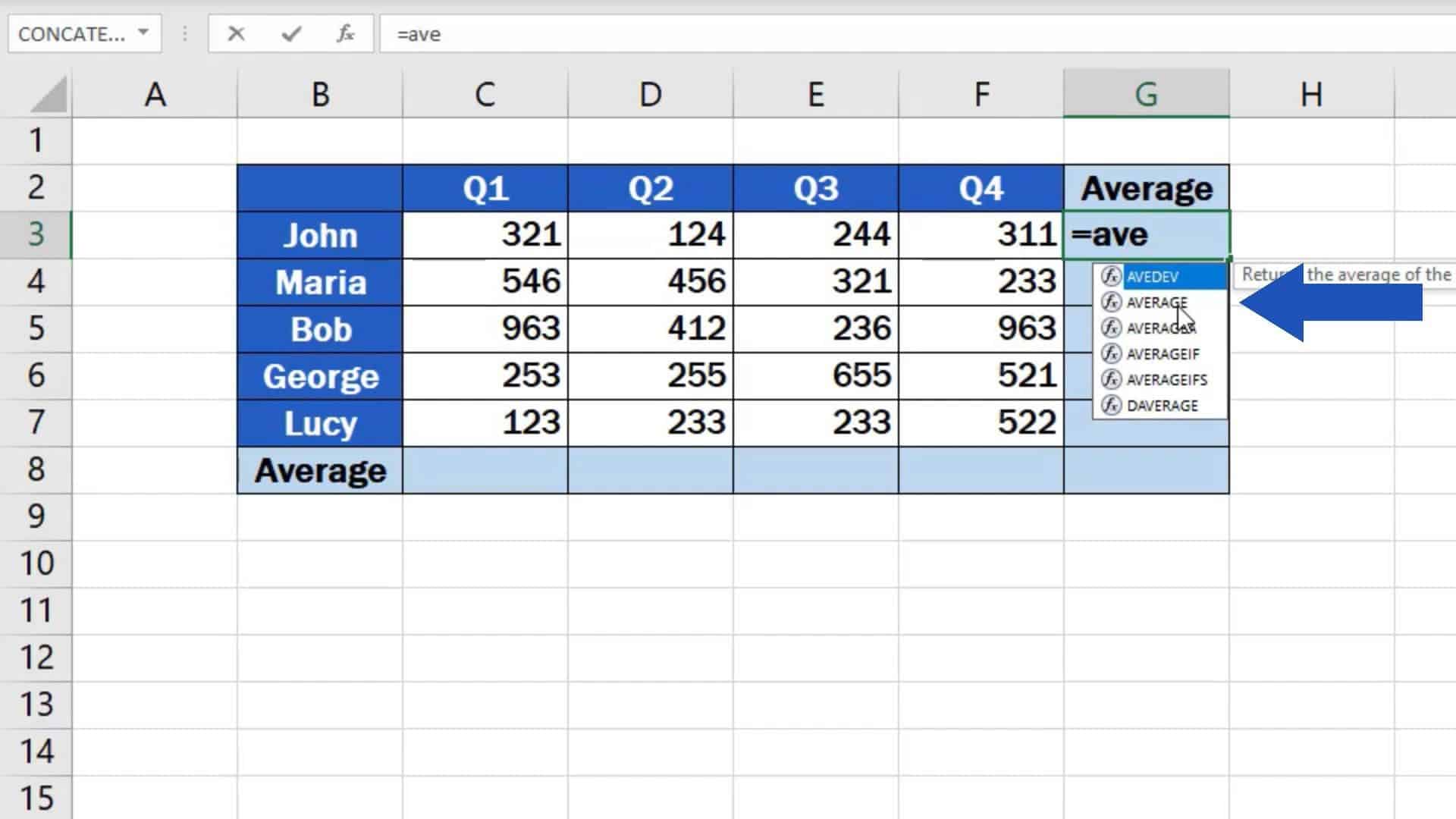
Okay, grab your coffee. Here’s the magic trick. Type this into a cell: =AVERAGE(. See? You’re already doing it. Now highlight the cells you want to average. Close the parenthesis. Hit Enter.
Boom. Excel spits out the average like it’s nothing. Nothing. It’s like having a tiny robot do your boring math. And that robot never complains.
Let’s say you have numbers in cells A1 through A10. Your formula looks like this: =AVERAGE(A1:A10). Go ahead. Try it. I’ll wait. (Sips coffee.)
But Wait—What About Blanks and Errors?
Oh, you’ve got blanks? Excel ignores them. How nice of it. Same with cells that have text. It just skips right over them like they don’t exist. Very polite.
But errors? Like a #DIV/0! or #N/A? Those will break your average. The function throws its hands up and says, “Nope, I’m out.” So clean up your errors first, friend. Or use =AGGREGATE(1,6,range) to ignore errors. But that’s advanced nerd stuff.